using LinearAlgebra, StatsBase, Statistics
using SparseArrays
using BenchmarkTools
using Plots, StatsPlots
using EcologicalNetworks
Networks are (more or less) diagonal
In part 1 and part 2 of this posts series we introduced and explored the notion of diagonality for networks. Roughly put, a network is diagonal if most of his interactions fall on the diagonal of the networks’ adjacency matrix. In the square world (unipartite networks) this is quite straightforward, as we have a natural notion of diagonal and a following distance from it. In the rectangular world (bipartite networks) this is a bit more hard to obtain. The “raw” diagonality metric depends on the specific matricial representation of the network, that is, on the choice of labelling order for the nodes in the network. Taking this into account, the diagonality we consider is (1) the highest “raw” diagonality we can get for a given network by swapping the columns’ and rows’ order, (2) normalised by the highest possible diagonality for a matrix with a given amount of links.
I promised I was going to explore some real example, and see if they are more or less diagonal than one can think, maybe infer some interesting ecological insight.
Bug bug bugging
Yet, I am really not done yet with the preliminary work.
Two things have been bugging me since last time. Two things I tried to ignore, but came back biting me.
Size (in)variance
The first is that k and α in the original definition were absolute values. This meant that the “band” around the diagonal was relatively narrower for larger networks. And, thus, the diagonality score for larger networks was going to be smaller by definition. Which made for nice plots like the one at the end of part 2. But also meant that any result we were going to find was almost surely driven by the shear size of the network. So, yeah, we don’t want it.
We want the diagonality score to be indipendent of the network size.
Random walkers don’t win marathons
The second problem comes from the fact that we do have a quite big space to traverse in order to get to the goal. What makes it even more unnerving, is that we are trying to traverse it blind (and drunk). We do a random step swapping some column (or row), check if we got closer to our destination, step back if we didn’t. As long as our matrix is small, with enough steps and reshuffle, we have a some chance of getting there. When we have some hundred columns and rows, we are doomed.
To give an idea, in 10×8 network we have
factorial(10) * factorial(8)146313216000
possible choices. For a 100×120 network we have
factorial(big(100)) * factorial(big(120))624305990113445326111717238107680430805551283706623610095858093543562860969
096225519257072922595371956315781347805727783764270902475511655549958618349
952024266237377337115021869528529962853910482352006491591894648711476607201
534331879629342355561291393113660099776974487582843277583259098376524923341
373440000000000000000000000000000000000000000000000000000
possible choices. That number is also known as “nope-nope-no-way”. Testing some 100 thousands combinations would lead us nowhere.
The result is that larger networks are even more penalized.
Improving resolutions
Luckily, we have some solutions. The first, for the size dependency, has been suggested by Rogini Runghen, my PhD student; the other, to explore the space in a more efficient way, by my University of Canterbury;s colleague, Thomas Li.
Relative theory
What we need is to make k a relative quantity, instead of an absolute one. So, instead of
considering the absolute distance from the diagonal, we normalise the distance so
that at most is 1. Than we can simply read k=0.2 as “consider the entries up to
20% of the maximum distance from the diagonal”.
Squint your eyes
If you can’t solve the hard problem, solve an easy one. If it is true that we can’t easily solve a 100×120 network optimization, it is als true that solving 2×2 problem is embarassingly easy. A 2×2 has just 4 possible choices, and thus we can exhaustively search it. And, actually, it does not seem to hard even to solve exhaustively a 5×5 one (with 14400 possible choices).
If we can squint the eyes and see our network as a 5×5 one, than we can start from that solution, increasing the resolution a bit at a time, and improve from there. We can, in other fancier words, adopt a hierarchical approach, using a series of grids with increasing resolution.
As I’m writing…
Working on this two problems, I also realised there was a third, slight, improvement I could make.
In the original version of the second post, I was asking Julia to work directly on the rows and columns of the matrices. That is, copying and rewriting. What we actually need to do is less demanding than that. Instead of working on the arrays, we can work on their indexes. That has the additional feature of always preserving the integrity of rows and nature (we do not risk to mess up the network). And because we limit ourselves to just swap indexes, we can skip all the checks that Julia does to be sure we are not trying to access the matrix outside its bounds.
State of my art
So, where am I at with the plan?
A couple of things are done, one is hard.
Producing a relative version for the α and k was the easiest thing to implement, once I knew what I wanted.
And playing with Pluto.jl to have a live update of the tweaking has been a great experience.
Rectangles Never Change, Oi!
The new diagonality_scores() function is as follows:
fancy = (x,y,I,J) -> abs.(round.(((J.*x).-(I.*y))/sqrt(I*J)))

function diagonal_scores(
        I::T, J::T,
        α::F = 0.1, k::F = 0.2;
        f::D = fancy) where {T <: Int, F <: Number, D <: Function}

    Mdists = Array{Float64}(undef,I,J)

    for i in 1:I, j in 1:J
       @inbounds Mdists[i,j] = f(i,j,I,J)
    end

	Mdists .*= maximum(Mdists)^(-1)
	Mdists .= α.^Mdists
	Mdists[Mdists .< α^k] .= 0

    return sparse(Mdists)
end
diagonal_scores (generic function with 3 methods)
And we can easily see that it is indeed size invariant:
plot(layout = (2,2),
    heatmap(Matrix(diagonal_scores(17,15)), title = "17×15", xticks=false, yticks=false, legend=false),
    heatmap(Matrix(diagonal_scores(50,70)), title = "50×70", xticks=false, yticks=false, legend=false),
    heatmap(Matrix(diagonal_scores(170,150)), title = "170×150", xticks=false, yticks=false, legend=false),
    heatmap(Matrix(diagonal_scores(500,700)), title = "500×700", xticks=false, yticks=false, legend=false),
)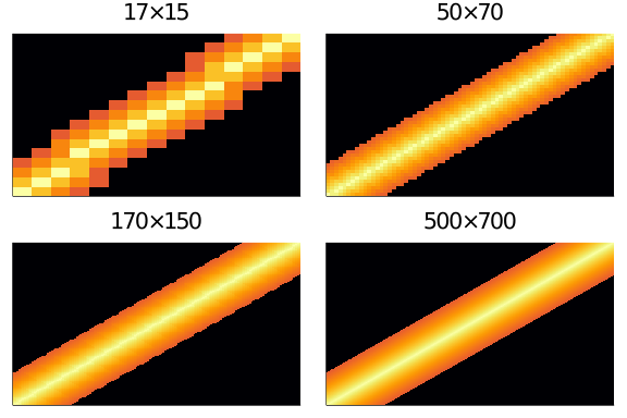
As the size increases, the heatmap become more finely defined, but stays substantially the same.
That’s a beuty, isn’t it?
Do the Permute, Do the View
Avoiding to rewrite everything is promising, but opens the door to a number of choices. I’m trying to benchmark and benchmark and benchmark to see what works faster. I would have been quicker had I known more robustly how views and memory allocation and that stuff actually works, for real.
The crucial step here happened within the optim_diag() function. If we were working on
the rows, we would have done something like:
x, y = sample(1:I,2,replace = false)
M[x,:], M[y, :] = M[y, :], M[x, :]
where I is the number of rows in the matrix M. Then we tested whether the improvement
in the diagonality score was worth the swap by evaluating
Δstate = (diag_here(M)-target)^power_ofIf the improvement was enough, we were done; otherwise we would have step back doing that step one more time:
M[x,:], M[y, :] = M[y, :], M[x, :]This operations are probably cheap enough in small matrices, but my fear is that they become expensive in large matrices.
Instead, let Ix and Jx be the index arrays for the matrix we are working on. What we want to do is evaluating
x, y = sample(1:I,2,replace = false)
diag_here(M[swap(Ix,x,y),Jx])
where swap(Ix,x,y) is the array Ix where the x and y positions are swapped. If the swap pass the test it’s
fine, otherwise we swap them back.
Now, I’m not sure I know what’s the fastest way of doing swapping of element positions in an array. If you got suggestion, hit me!
function swap!(Xx::A,to_swap)::A where {A<:AbstractArray}
    Xx[to_swap] = Xx[reverse(to_swap)]
end
swap! (generic function with 1 method)
Finally, the crucial step can be done by either reading the rows (or columns) in the right order or by using
something like permute() that works for permuting sparse matrices (luckily, our networks are sparse).
We can code up three different version and benchmark to see what’s faster.
function read_and_rewrite!(M)
    I, J = size(M)
    Ix, Jx = collect(1:I), collect(1:J)
    for _ in 1:1000
        to_swap = sample(Ix,2,replace = false)
        @inbounds M[to_swap[1],:], M[to_swap[2], :] = M[to_swap[2], :], M[to_swap[1], :]
        sum(M) # any function would do here
    end
    return(M, Ix, Jx)
end

function read_swapped(M)
    I, J = size(M)
    Ix, Jx = collect(1:I), collect(1:J)
    for _ in 1:1000
        to_swap = sample(1:I,2,replace = false)
        swap!(Ix,to_swap)
        sum(M[Ix,:]) # any function would do here
    end
    return(M, Ix, Jx)
end

function permute_and_compute(M)
    I, J = size(M)
    Ix, Jx = collect(1:I), collect(1:J)
    for _ in 1:1000
        to_swap = sample(1:I,2,replace = false)
        swap!(Ix,to_swap)
        sum(permute(M,Ix,Jx)) # any function would do here
    end
    return(M, Ix, Jx)
end
permute_and_compute (generic function with 1 method)
We get ourselve a matrix to test the three approaches upon:
Observed_Network = simplify(convert(BipartiteNetwork, web_of_life(web_of_life()[10].ID)))
Msp = sparse(Int.(Observed_Network.A))
31×18 SparseArrays.SparseMatrixCSC{Int64,Int64} with 88 stored entries:
[1 , 1] = 1
[2 , 1] = 1
[3 , 1] = 1
[4 , 1] = 1
[6 , 1] = 1
[8 , 1] = 1
[9 , 1] = 1
[10, 1] = 1
[16, 1] = 1
⋮
[20, 14] = 1
[7 , 15] = 1
[14, 15] = 1
[4 , 16] = 1
[11, 16] = 1
[1 , 17] = 1
[7 , 17] = 1
[11, 17] = 1
[14, 17] = 1
[6 , 18] = 1
rr_results = @benchmark read_and_rewrite!($Msp);
rs_results = @benchmark read_swapped($Msp);
pc_results = @benchmark permute_and_compute($Msp);
The results are:
rr_resultsBenchmarkTools.Trial:
memory estimate: 21.86 MiB
allocs estimate: 43912
--------------
minimum time: 8.959 ms (0.00% GC)
median time: 11.755 ms (13.04% GC)
mean time: 10.557 ms (14.82% GC)
maximum time: 14.436 ms (22.68% GC)
--------------
samples: 474
evals/sample: 1
rs_resultsBenchmarkTools.Trial:
memory estimate: 11.32 MiB
allocs estimate: 15002
--------------
minimum time: 13.059 ms (0.00% GC)
median time: 13.235 ms (0.00% GC)
mean time: 14.037 ms (5.43% GC)
maximum time: 19.160 ms (19.08% GC)
--------------
samples: 357
evals/sample: 1
pc_resultsBenchmarkTools.Trial:
memory estimate: 18.49 MiB
allocs estimate: 11002
--------------
minimum time: 5.664 ms (0.00% GC)
median time: 5.884 ms (0.00% GC)
mean time: 7.045 ms (16.93% GC)
maximum time: 9.395 ms (31.90% GC)
--------------
samples: 710
evals/sample: 1
And finally we plot what we found to see what works best.
boxplot(rr_results.times, lab = "read_and_rewrite!", ylims = (0,Inf))
boxplot!(rs_results.times, lab = "read_swapped")
boxplot!(pc_results.times, lab = "permute_and_compute")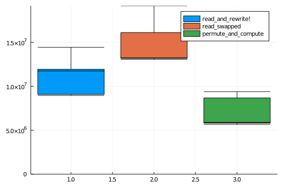
So, yeah, the permute_and_compute() saves us some time, but not that much.
Interesting, the read_swapped() approach is actually slower than the one
based on reading and rewriting.
Thus, we can redefine our optimization function according to our discover.
function optim_diag(M::T;
                    α = 0.25, k = 0.2, f = fancy,
                    λ = 0.999, t0 = 2.0,
                    Nsteps = 10000) where {T <: AbstractMatrix}

    Matrix_of_Scores = diagonal_scores(size(M)...,α,k,f = f)
    Norm_factor = normalize_score(sum(M), value_count(Matrix_of_Scores))

    diag_here(Matr) = normalized_diagonality(Matr, Matrix_of_Scores, Norm_factor)
    Δbest = (diag_here(M)-1.1)^2.0

    I, J  = size(M)
    Ix, Jx = collect(1:I), collect(1:J)

    for step in 1:Nsteps
        t = λ^(step-1)*t0
        # we work on either rows or columns at random
        if rand() < I/(I+J) # work on rows
            to_swap = sample(1:I,2,replace = false)
            swap!(Ix,to_swap)
            Δstate = (diag_here(permute(M,Ix,Jx))-1.1)^2.0
            Δ = Δstate - Δbest
            P = exp(-Δ/t)
            if (rand() ≤ P) & (all(values(degree(M)) .> 0.0))
                Δbest = Δstate
            else
                swap!(Ix,to_swap)
            end
        else
            to_swap = sample(1:J,2,replace = false)
            swap!(Jx,to_swap)
            Δstate = (diag_here(permute(M,Ix,Jx))-1.1)^2.0
            Δ = Δstate - Δbest
            P = exp(-Δ/t)
            if (rand() ≤ P) & (all(values(degree(M)) .> 0.0))
                Δbest = Δstate
            else
                swap!(Jx,to_swap)
            end
        end
    end
    return (Ix, Jx)
end
optim_diag (generic function with 1 method)
To mesh is to mess
The adoption of mesh-refinement optimization (or, if one prefers, multiresolution grids) is still heavily work in progress.
I have coded up a function to blur my sight and reduce the resolution of the adjacency matrix I’m working on.
function lower_resolution(
        Matr::M,
        Rows::I, Columns::I,
        Rtresolution::N, Ctresolution::N
        ) where {M<:AbstractMatrix, I<:AbstractArray, N<:Int}

    Is, Js = size(Matr)

    I_chunks = collect(Iterators.partition(Rows, cld(Is,Rtresolution)))
    J_chunks = collect(Iterators.partition(Columns, cld(Js,Ctresolution)))
    Rresolution, Cresolution = length(I_chunks), length(J_chunks)

    Low_dim = Array{Int64}(undef,Rresolution,Cresolution)

    for iₗ in 1:Rresolution, jₗ in 1:Cresolution
      @inbounds  Low_dim[iₗ, jₗ] = sum(Matr[Rows[I_chunks[iₗ]],Rows[J_chunks[jₗ]]])
    end

    return Low_dim
end
lower_resolution (generic function with 1 method)
We can use lower_resolution() to produce a low resolution version of some input matrix:
plot(
    heatmap(Matrix(Msp), title = "Full resolution"),
    heatmap(Matrix(lower_resolution(Msp,1:31,1:18,2,2)), title = "2×2"),
    heatmap(Matrix(lower_resolution(Msp,1:31,1:18,3,3)), title = "3×3"),
    heatmap(Matrix(lower_resolution(Msp,1:31,1:18,6,4)), title = "6×4")
)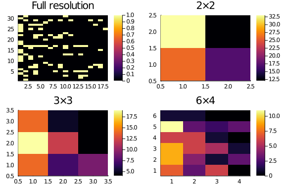
Solving the lower resolution problems first is going to be much easier, and should bring us much closer to a decent solution. In the next days the project is to clean up the mesh refinement optimization.
Things that require some focus are:
1. keeping track of the indexes across the resolution levels: when we swap at
one level, we need to swap also at the finer levels accordingly.
2. the normalize_score() function was meant for binary (0,1) matrices. Now,
we need to extend it to work on lower resolution matrices which entries are the
sum of the higher resolution ones. Thus, they are no more binary.