using LinearAlgebra, StatsBase, Statistics
using Plots
using EcologicalNetworks

The story: where we have left it?

In part 1 of this posts series on network diagonality we wrapped up by writing two functions that compute the raw and normalised diagonality for a specific representation of a network in terms of its adjacency matrix.

function raw_diagonality(M::T, α::Float64 = 0.25, k::Int = 6) where T <: Matrix
    return sum(M .* diagonal_scores(size(N)[1],α,k))
end

function raw_diagonality(N::T; α::Float64 = 0.25, k::Int = 6) where T <: UnipartiteNetwork
    return raw_diagonality(N.A, α = α, k = k)
end

function norm_diagonality(M::T, α::Float64 = 0.25, k::Int = 6, norm_function::F = sum) where {T <: Matrix, F <: Function}
    return sum(M .* diagonal_scores(size(N)[1],α,k)) / norm_function(M)
end

function norm_diagonality(N::T; α::Float64 = 0.25, k::Int = 6, norm_function::F = sum) where  {T <: Matrix, F <: Function}
    return norm_diagonality(N.A, α = α, k = k, norm_function = norm_function)
end

norm_diagonality (generic function with 4 methods)

The functions rely on the notion of distance from the diagonal for the entry of a square matrix.

diag_dist = (x,y) -> abs.(x .- y)

function diagonal_scores(Msize::T, α::F = 0.25, k::T = 3) where {T <: Int, F <: Number}
    Mdists = Array{Float64}(undef, Msize, Msize)
    for i in 1:Msize
        Mdists[i,:] .= α .^ diag_dist(i,1:Msize)
    end
    Mdists[Mdists .< α^k] .= 0
return Mdists 
end

diagonal_scores (generic function with 3 methods)

Importantly, we identified three things we’ll need to take care of moving into the realm of rectangular matrices.

The Rectangular diagonal is not the square one.
We need to be careful with our normalization.
And remember that representation matter.

The rectangular diagonal

The diagonal distance we defined in part 1 is based on the notion that the straight line defined by $y-x = 0$ (that is, $y = x$), in the finite geometry of the matrix entries coordinates, is indeed the matrix diagonal.

That’s not so simple in a bipartite network where the numbers of rows and columns differ. Entries Aᵢᵢ in the adjacency matrix of a bipartite network do not have any special meaning because the left ᵢ and the right ᵢ refer to two different set of species (taxa, individuals, or nodes in general). Thus, the usual definition of diagonal is not much relevant.

What we are after is, more vaguely, a rectangular matrix that looks like a diagonal square matrix, when we squeeze and push and press into a square our rectangle. Alas!, we can not transform the rectangular matrix into a square one without dropping or aggregating some species. And we don’t want that.

Well, no biggie. We can still go back to elementary school and draw a diagonal in a rectangle. Let capital $I$ be the number of rows and capital $J$ be the number of columns in the matrix. We can write an equation for the diagonal modifying the square one. Roughly speaking, the diagonal will be the line for which $\frac{J}{I}x - y = 0$. Or, that should be the same $Iy - Jx = 0$ (that is, $Iy = Jx$). For each step in the $x$ direction, we go a $\frac{J}{I}$th of a step in the $y$ direction. And because we are working with a discrete geometry (the entries of the adjacency matrix), we will need to round it up to integer values. Or take the ceiling, or the floor.

Something like this should do:

rect_diag_dist = (x,y,I,J) -> abs.(round.(J/I .* x .- y))

#5 (generic function with 1 method)

or this

rect_diag_dist_2 = (x,y,I,J) -> abs.(round.(J/I .* x) .- y)

#7 (generic function with 1 method)

or this

rect_diag_dist_3 = (x,y,I,J) -> abs.((J .* x) .- (I.* y))

#9 (generic function with 1 method)

One would hope that this somewhat equivalent expression versions of the diagonal would be mathematically equivalent and give the same scores. Spoiler, they don’t. Remember: things are weird in rectangular world.

Having a rectangular diagonal distance, we can define the diagonal scores of rectangular matrices.

function diagonal_scores(Isize::T, Jsize::T,
        α::F = 0.25, k::T = 4;
        f::D = rect_diag_dist) where {T <: Int, F <: Number, D <: Function}
    Mdists = Array{Float64}(undef, Isize, Jsize)
    dist_diag = (x,y) -> f(x,y,Isize,Jsize)
    for i in 1:Isize
            Mdists[i,:] .= α .^ dist_diag(i,1:Jsize)
    end
    Mdists[Mdists .< α^k] .= 0
return Mdists 
end

diagonal_scores (generic function with 6 methods)

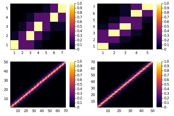
And they do look like what we would expect. Let’s consider a 50×70 matrix.

heatmap(diagonal_scores(50,70,0.6,6))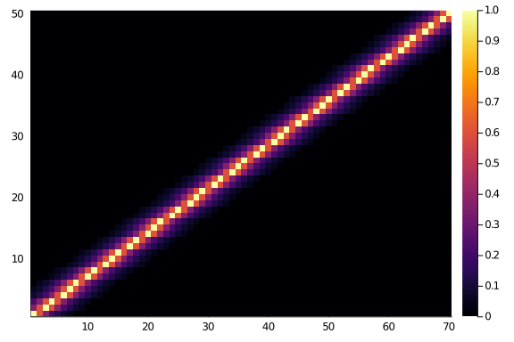

And, if we look at a 70×50 matrix we will surely see the same thing, as symmetry and beauty and order. Right?

Where’s your symmetry now?

heatmap(diagonal_scores(70,50,0.6,6))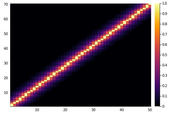

Ok, well, maybe it’s just a glitch, let’s see side by side, and maybe with a smaller matrix

plot(
heatmap(diagonal_scores(5,7,0.25,2)),
heatmap(diagonal_scores(7,5,0.25,2))
)

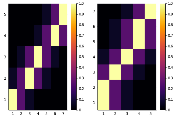
Oh nooo. That’s even worse. The two score matrices are not the same. Do they have, at least, the same total scores?

println(sum(diagonal_scores(5,7,0.25,2)))
println(sum(diagonal_scores(7,5,0.25,2)))

7.4375
10.25

No, they do not. And that’s that. We can try to do better, maybe by using some fancy function. I spent some hours looking for some ingenious trick, and failed. The fanciest I got was using the geometric mean of $I$ and $J$. The geometric mean!

fancy = (x,y,I,J) ->
                abs.(round.(((J .* x) .- (I.* y)) / (sqrt(I * J))))

#14 (generic function with 1 method)

Which look like this:

plot(
heatmap(diagonal_scores(5,7,0.25,2, f = fancy)),
heatmap(diagonal_scores(7,5,0.25,2, f = fancy)),
heatmap(diagonal_scores(50,70,0.6,8, f = fancy)),
heatmap(diagonal_scores(70,50,0.6,8, f = fancy))
)

And should be (more?) symmetric.

sum(diagonal_scores(50,70,0.25,2, f = fancy)) == sum(diagonal_scores(70,50,0.25,2, f = fancy))

true

If you do better than this, please let me know!

For a blog post, is enough, I reckon: Problem 1 is fixed

A tighter normalization

We noticed in part 1 that using the number of interactions present in the network as the denumerator of our normalization is not the super precise. Indeed, not all interaction can achieve the maximum score, as the number of available seats at the high table (the number of matrix entries that would get the maximum score) is limited.

So, how many entries can get the maximum score (and the other scores)? In the square world, it’s easy. If you have N species, then N entries in the greater diagonal, 2×(N-1) for the entries a step away, 2×(N-2) for the ones one step further, and so on.

It’s NOT so easy, and it depends on the fine details of the problem, for the rectangular world. The exact matrix dimension and the diagonal distance function we use matters.

Too lazy to figure out an analytic a priori solution, we just count.

function value_count(M::T) where T <: Matrix
    sort(countmap(vec(M)), rev = true)
end

value_count (generic function with 1 method)

Compare for example

value_count(diagonal_scores(50,70,0.25,2, f = fancy))

OrderedCollections.OrderedDict{Float64,Int64} with 4 entries:
  1.0    => 50
  0.25   => 118
  0.0625 => 116
  0.0    => 3216

and

value_count(diagonal_scores(51,70,0.25,2, f = fancy))

OrderedCollections.OrderedDict{Float64,Int64} with 4 entries:
  1.0    => 59
  0.25   => 118
  0.0625 => 116
  0.0    => 3277

Don’t you also find upsetting that adding 1 rows adds 9 maximum score entries? Yes, yes you do. We hate it, for good reasons. But, ok, as long as Julia does the counting, who cares.

The next step requires to fill in the available entries with the links present in the network.

To compute the score normalization we need two things: the number of links, and the counts of the score values.

function normalize_score(L::T,CountedValues) where T <: Int
    Tot_links = L
    nz_scores, nz_seats = CountedValues.keys, CountedValues.vals
     
    d = 1
    score = 0
    while (Tot_links >= nz_seats[d]) && d < length(nz_seats)
        Tot_links -= nz_seats[d]
        score += nz_seats[d] *  nz_scores[d]
        d += 1
    end
    if d < length(nz_seats)
        score += nz_scores[d] *  Tot_links
    end
    return score
end

normalize_score (generic function with 1 method)

Now, from the adjacency matrix A of a network N, we can get all the necessary information bits to compute the maximum possible diagonality score.

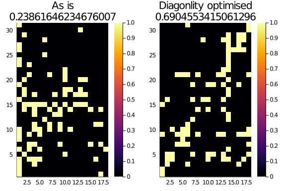
Let’s try on a real ecological bipartite network, for example, this host-parasite network:

web_of_life()[10]

(ID = "A_HP_010", Species = 49, Interactions = 88, Connectance = 0.158, Typ
e_of_interactions = "Host-Parasite", Type_of_data = 1, Reference = "Hadfiel
d JD, Krasnov BR, Poulin R, Shinichi N (2013) A tale of two phylogenies: co
mparative analyses of ecological interactions. The American Naturalist 183(
2): 174-187", Locality_of_Study = "East Balkhash", Latitude = 46.166667, Lo
ngitude = 74.333333)

We obtain it from the Web of Life and convert it in a network.

Observed_Network = simplify(convert(BipartiteNetwork, web_of_life(web_of_life()[10].ID)))

31×18 bipartite  ecological network (Bool, String) (L: 88)

The network adjacency show some diagonal structure, but not an awful lot.

Observed_Network.A |> heatmap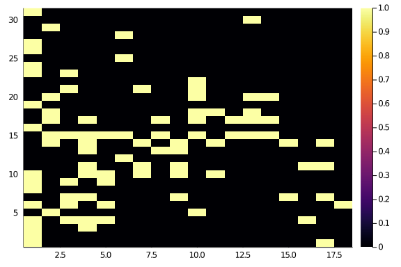

Let’s compute the normalized diagonality for the network.

Matrix_of_Scores = diagonal_scores(
        size(Observed_Network)...,
        0.6,8,
        f = fancy)
Observed_Score = Observed_Network.A .* Matrix_of_Scores |>
        sum
Normalization = normalize_score(
    links(Observed_Network),
    value_count(Matrix_of_Scores))
Normalised_Score = Observed_Score / Normalization

0.35281167688022286

Or for the butterfly and moths network:

butterflies = Bool.(zeros(12,12) + I)
Matrix_of_Scores = diagonal_scores(
        size(butterflies)...,
        0.6,8,
        f = fancy)
Observed_Score = butterflies .* Matrix_of_Scores |>
        sum
Normalization = normalize_score(
    sum(butterflies),
    value_count(Matrix_of_Scores))
Normalised_Score = Observed_Score / Normalization

1.0

imperfections = Bool.(round.(rand(size(butterflies)...) .* 0.6))
moths = butterflies .⊻ imperfections
Matrix_of_Scores = diagonal_scores(
        size(moths)...,
        0.6,8,
        f = fancy)
Observed_Score = moths .* Matrix_of_Scores |>
        sum
Normalization = normalize_score(
    sum(moths),
    value_count(Matrix_of_Scores))
Normalised_Score = Observed_Score / Normalization

0.6137534171428571

Wrap it up

We can define a function doing this job for us.

function normalized_diagonality(N::T; α, k, f = fancy)::Float64 where {T <: DeterministicNetwork}
    Scores = diagonal_scores(size(N)..., α,k,f = f)
    Observed_Score = sum(N.A .* Scores)
    Normalization = normalize_score(links(N), value_count(Scores))
    return (Observed_Score / Normalization)
end

normalized_diagonality (generic function with 1 method)

Great, and it does not just work for the bipartite networks: it works also for rectangular ones for free.

So, can we set out to see how diagonal the world of ecological nets is?

Representation and order

Not so fast!

We still have one challenge to solve. Namely, the order in which we decided to label the species does affect the diagonality score we compute. Changing the order of rows, and changing the order of columns in the matrix will give different diagonality values.

We don’t want that. We want the score to be independent of any arbitrary decision we took when representing it as an adjacency matrix. That is, we want it to be an intrinsic graph property.

But all our code depends on this order, and I’ve no idea how to compute the score not relying on a particular matrix representation (any idea? it may well be the case that this is actually possible!). Thus, we are going the lazy way, and brute force our way through.

In particular, we are going to use some crude simulated annealing to compute the maximum diagonality score between all the possible representations of our observed networks in terms of adjacency matrix.

The base idea here is to swap rows and columns until we get to a better result. With a bit of lucky, and a bit of randomness, we can get to the maximum (or close to it).

One thing to notice is that when we shuffle the order of rows and columns certain things stay the same. The matrix of diagonal scores depends only on the size of the observed matrix, α, and k; the normalization factor depends on then value count of the matrix of diagonal scores and the number of links in the observed network. Thus, we don’t need to recompute this objects every time we reshuffle the network. Let’s write a slightly more convenient normalized_diagonality then:

function normalized_diagonality(N::T, Scores::M, Normalization::S) where {T <: DeterministicNetwork, M <: Matrix, S <: Number}
    Observed_Score = sum(N.A .* Scores)
    return Observed_Score / Normalization
end

normalized_diagonality (generic function with 2 methods)

Now, annealing! Here I rely heavily on some Timothée and Tanya’s code from a forthcoming paper.

function optim_diag(N::T; α = 0.25, k = 3, f = fancy,
                    λ = 0.999, t0 = 2.0, Nsteps = 10000) where {T <: BipartiteNetwork}

    Matrix_of_Scores = diagonal_scores(size(N)...,α,k,f = f)
    Norm_factor = normalize_score(links(N), value_count(Matrix_of_Scores))

    diag_here(Net) = normalized_diagonality(Net, Matrix_of_Scores, Norm_factor)
    Δbest = (diag_here(N)-1.1)^2.0
    
    M = copy(N)
    rows, columns = richness(M, dims = 1), richness(M, dims = 2)

    for step in 1:Nsteps
        t = λ^(step-1)*t0
        # we work on either rows or columns at random
        if rand() > 0.5 # work on rows
            from = rand(1:rows)
            to = rand(1:rows)
            M.A[from,:], M.A[to, :] = M.A[to, :], M.A[from, :]
            Δstate = (diag_here(M)-1.1)^2.0
            Δ = Δstate - Δbest
            P = exp(-Δ/t)
            if (rand() ≤ P) & (all(values(degree(M)) .> 0.0))
                Δbest = Δstate
            else
                M.A[from,:], M.A[to, :] = M.A[to, :], M.A[from, :]
            end
        else
            from = rand(1:columns)
            to = rand(1:columns)
            M.A[:,from], M.A[:,to] = M.A[:,to], M.A[:,from]
            Δstate = (diag_here(M)-1.1)^2.0
            Δ = Δstate - Δbest
            P = exp(-Δ/t)
            if (rand() ≤ P) & (all(values(degree(M)) .> 0.0))
                Δbest = Δstate
            else
                M.A[:,from], M.A[:,to] = M.A[:,to], M.A[:,from]
            end
        end
    end
    return M
end

optim_diag (generic function with 1 method)

This tiny monster of a function gets a network and some parameters as input and return the most diagonal representation of that network. We can see it in action on our bipartite ecological network:

Optimised_M = optim_diag(Observed_Network, k = 3)
plot(
    heatmap(Observed_Network.A, title="As is\n$(normalized_diagonality(Observed_Network, α = 0.25, k = 3))"),
    heatmap(Optimised_M.A, title="Diagonlity optimised\n$(normalized_diagonality(Optimised_M, α = 0.25, k = 3))")
)

We are almost there. The only remaining risk is that the optim_diag function can get stuck in local optima. To avoid that, instead of running it just once, we run it a few times, reshuffling the observed network before each time.

function shuffle(N::T) where {T <: BipartiteNetwork}
    I, J = richness(N, dims = 1), richness(N, dims = 2)
    reorder_rows = sample(1:I, I, replace = false)
    reorder_cols = sample(1:J, J, replace = false)
    A = N.A[reorder_rows,reorder_cols]
    return BipartiteNetwork(A)
end

shuffle (generic function with 1 method)

Wrapping everything up for bipartite networks:

function diagonality_score(N::T;
                           α::F = 0.25, k::Int = 3, f = fancy,
                           λ = 0.999, t0 = 2.0,
                           repeats::Int = 10,
                           return_M::Bool = false
                           ) where {T <: BipartiteNetwork, F <: Number}
    
    Nsteps = k * 10000
    repeats = k * repeats

    Matrix_of_Scores = diagonal_scores(size(N)...,α,k,f = f)
    Norm_factor = normalize_score(links(N), value_count(Matrix_of_Scores))

    diag_here(Net) = normalized_diagonality(Net, Matrix_of_Scores, Norm_factor)
    optim_here(Net) = optim_diag(Net, α = α, k = k, f = f, λ = λ, t0 = t0, Nsteps = Nsteps)
    
    M = optim_diag(N, α = α, k = k, f = f, λ = λ, t0 = t0, Nsteps = Nsteps)
    Diagonality = diag_here(M)
    for i in 1:repeats
        Ns = shuffle(N)
        Mtemp = optim_here(Ns)
        Diagonality_temp = diag_here(Mtemp)
        #@info Diagonality_temp, diagonality_here(Ns)
        if Diagonality_temp > Diagonality
            M, Diagonality = Mtemp, Diagonality_temp
        end
    end

    if return_M
        return (Diagonality = Diagonality, Web = M)
    else
        return (Diagonality = Diagonality)
    end
end

diagonality_score (generic function with 1 method)

Bipartite ecological networks are, indeed, diagonal

Warning, this does take a while. Probably there is ample space for code optimization.

Following the insight about the role of k and α from Diagonality part 1, we may want to scale them so that the diagonal scores are not too tight around the diagonal in larger networks. An heuristic may be to scale k with the log of the network richness.

webs = web_of_life()
nets = [simplify(convert(BipartiteNetwork, web_of_life(web.ID))) for web in webs]
diag_scores = [diagonality_score(net, α = 0.7, k = Int(round(log2(richness(net))))) for net in nets]

236-element Array{Float64,1}:
 0.8002280872475257
 0.7054857316332727
 0.8313281642989714
 0.8402029305733226
 0.8533270202020202
 0.7308735644876326
 0.8604773238983596
 0.8411049469964665
 0.7604536193379082
 0.7431291117656179
 ⋮
 0.9588235294117649
 0.940586637150332
 0.9146963806603515
 0.9152941176470588
 0.9155434782608695
 0.7776398058252427
 0.9166581956797966
 0.7883033149171271
 0.5464421119556765

(Note to self: the previous step is massively parallelisable, so, do that!)

Yay! We can finally plot a diagonality distribution

histogram(diag_scores,
    ylab = "frequency", xlab = "diagonality score",
    title = "Bipartite ecological networks are heavily diagonal",
    bins = 0.0:0.05:1.0)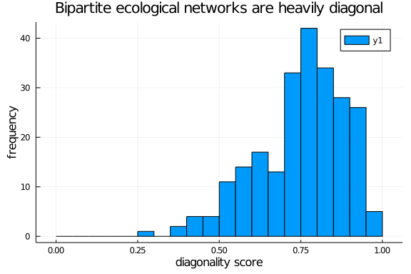

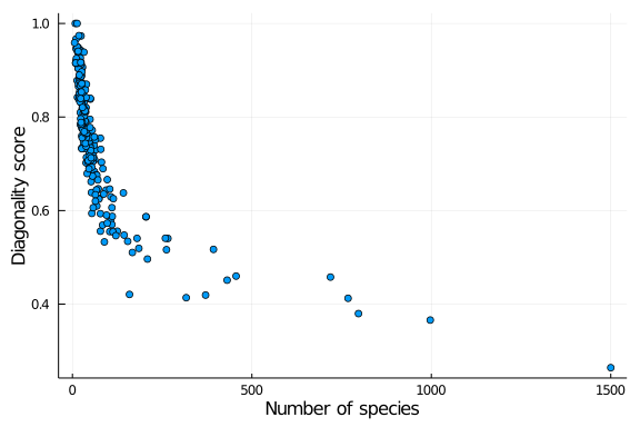
and explore how diagonality is distributed across other network properties, such as the number of species in the web:

scatter(richness.(nets), diag_scores,
        lab = "",
        xlab = "Number of species", ylab = "Diagonality score")