using LinearAlgebra, StatsBase, Statistics
using Plots
using EcologicalNetworks

Of butterflies, “moths” and flowers

In the last year or so I’ve spent a peculiar amount of time thinking about how much the ecological (or ecology-adjacent) networks I was working with were “diagonal”. How many of the interactions fall on, or nearby, the diagonal of the network’s adjacency matrix? I’ve been thinking about this because I have a hunch that some of favourite tools (namely, the ones based on the most wonderful of the matrix decomposition: the Singular Value decomposition) worked better on networks that were not heavily diagonal.

Yet, to be earnest, my working notion of “diagonality” was vague. I had in mind the pattern one would observe in an ecological network assembling under a regime of strong cospeciation (or coëvolution, codivergence, however you want to call it). For example, consider the cophylogeny drawn by Jennifer Hoyal Cuthill and Michael Charleston for 2012 paper on mimetic butterflies.

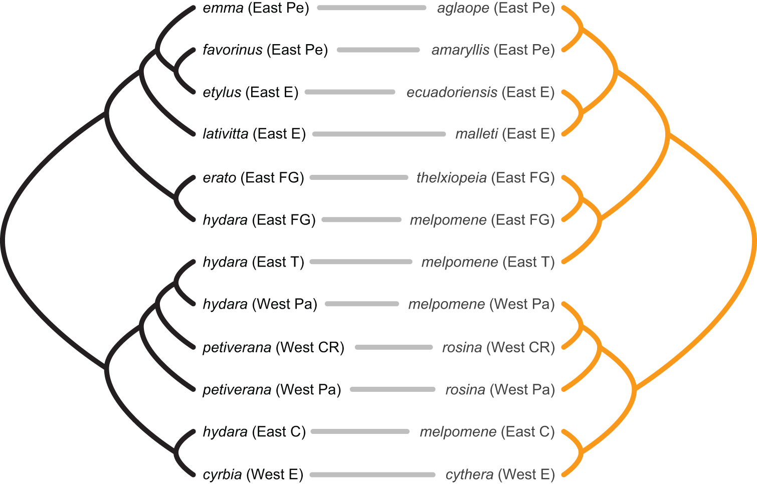
Labelling the taxa on the left side phylogeny as 1 to 12 and the right side ones as ‘a’ to ‘l’, Tte heatmap of the adjacency matrix of that network looks like a, you name it, diagonal:

butterflies = Bool.(zeros(12,12) + I)
heatmap(butterflies,
    xticks=(1:12),
    yticks=(1:12, string.(collect('a':'l'))))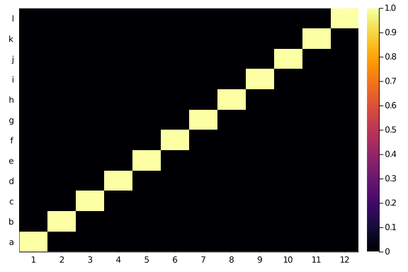

As some randomness is present in all biological processes, that is now we usually see when we plot ecological network. Yet, a lot of times is that plus some variability. Something like this:

imperfections = Bool.(round.(rand(size(butterflies)...) .* 0.6))
moths = butterflies .⊻ imperfections
heatmap(moths,
    xticks=(1:12),
    yticks=(1:12, string.(collect('a':'l'))))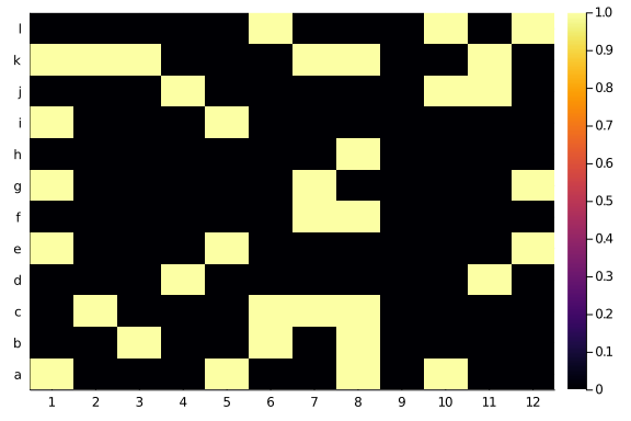

Put it roughly: the probability of observing an interaction decrease with the distance from the diagonal in the matrix. It seems like a little neat property to check for. My gut feeling is that most bipartite ecological networks would look a tad diagonal.

Here, I try to make my understanding more rigorous. I have three question I need an answer to. The first question is: can we measure the diagonality of a web? Let’s use the hive mind. The second is: how much diagonal are uni- and bi-partite ecological neworks? The third and last is: are the quality of my analytical tool affect by networks’ diagonality?

Here, I will start to answer question 1. But not all of, as it turns out to be harder, or more interesting, than expected.

Diagonal in a square world

Luckily, my call didn’t fall in the void.

Tim to the rescue

Timothée suggested to consider a Katz metric: we count the steps between the diagonal and the position in the matrix, and keep track of a score that is α^(number of steps) if there’s a link in that position or zero otherwise. He also suggests to normalise everything by the number of links present in the observed network.

pic.twitter.com/UTdtv9ekvV

— Dr. Timothée Poisot (@tpoi) November 4, 2020

Well, that does not look bad, and we can code it up!

Following Timothée, we first define a distance:

diag_dist = (x,y) -> abs.(x .- y)

#1 (generic function with 1 method)

And then we use it to see how far away an entry is from the diagonal.

We create a little function to explore the interplay between α and k in assigning the entries score.

function diagonal_scores(Msize::T, α::F = 0.25, k::T = 3) where {T <: Int, F <: Number}
    Mdists = Array{Float64}(undef, Msize, Msize)
    for i in 1:Msize
        Mdists[i,:] .= α .^ diag_dist(i,1:Msize)
    end
    Mdists[Mdists .< α^k] .= 0
return Mdists 
end

diagonal_scores (generic function with 3 methods)

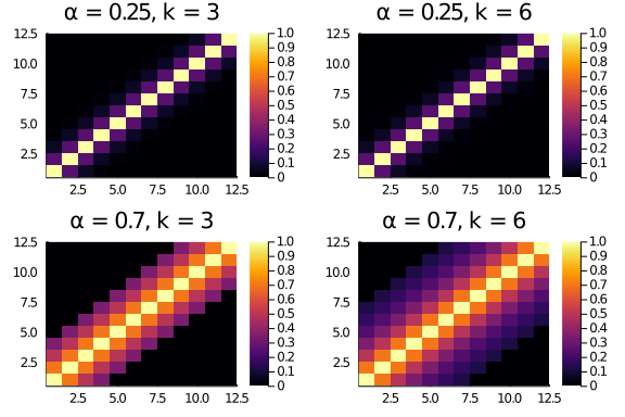
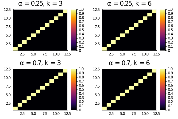
Tryin a couple of values for α and k, we see that a higher α flattens the scores (entries further away from the diagonal have a higher score).

plot(layout = (2,2),
    heatmap(diagonal_scores(12,0.25,3), title = "α = 0.25, k = 3"),
    heatmap(diagonal_scores(12,0.25,6), title = "α = 0.25, k = 6"),
    heatmap(diagonal_scores(12,0.7,3), title = "α = 0.7, k = 3"),
    heatmap(diagonal_scores(12,0.7,6), title = "α = 0.7, k = 6")
)

To get the score for a given adajcency matrix, we can simply multiply the adjacency by the diagonal scores matrix and sum up all entries.

Breaking it down in steps, for the butterflies matrix:

plot(layout = (2,2),
    heatmap(butterflies .* diagonal_scores(12,0.25,3), title = "α = 0.25, k = 3"),
    heatmap(butterflies .* diagonal_scores(12,0.25,6), title = "α = 0.25, k = 6"),
    heatmap(butterflies .* diagonal_scores(12,0.7,3), title = "α = 0.7, k = 3"),
    heatmap(butterflies .* diagonal_scores(12,0.7,6), title = "α = 0.7, k = 6")
)

As the butterflies matrix has entries only on the diagonal, nothing much interesting happens here. And in fact the scores will all be the same, no matter α and k.

println(sum(butterflies .* diagonal_scores(12,0.25,3)))
println(sum(butterflies .* diagonal_scores(12,0.25,6)))
println(sum(butterflies .* diagonal_scores(12,0.7,3)))
println(sum(butterflies .* diagonal_scores(12,0.7,6)))

12.0
12.0
12.0
12.0

BUT, for the “moths” adjacency matrix (that is, a slightly more noisy adjacency with entries outside the diagonal the distance and score parameters matter.

plot(layout = (2,2),
    heatmap(moths .* diagonal_scores(12,0.25,3), title = "α = 0.25, k = 3"),
    heatmap(moths .* diagonal_scores(12,0.25,6), title = "α = 0.25, k = 6"),
    heatmap(moths .* diagonal_scores(12,0.7,3), title = "α = 0.7, k = 3"),
    heatmap(moths .* diagonal_scores(12,0.7,6), title = "α = 0.7, k = 6")
)

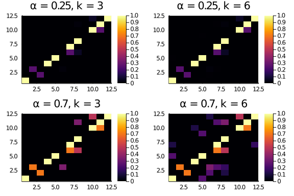
Indeed, the resulting scores are different:

println(sum(moths .* diagonal_scores(12,0.25,3)))
println(sum(moths .* diagonal_scores(12,0.25,6)))
println(sum(moths .* diagonal_scores(12,0.7,3)))
println(sum(moths .* diagonal_scores(12,0.7,6)))

9.15625
9.1826171875
12.466000000000001
14.713335999999998

So, the parameters matter (not surprisingly) and with “generous” enough scoring schemes (α = 0.7, k = 6) the raw diagonality score for the “moths” web is larger than the one for the butterflies (which is a bit unpleasant). We can “fix” this by normalising the raw scores in some way. Tim suggested to use the number of links present in the web.

This, matricially, corresponds to dividing by the total sum of the entries. Comparing the butterflies and “moths” matrix, we have a more reasonable result:

println(sum(butterflies .* diagonal_scores(12,0.7,3)) / sum(butterflies))
println(sum(butterflies .* diagonal_scores(12,0.7,6)) / sum(butterflies))
println(sum(moths .* diagonal_scores(12,0.7,3)) / sum(moths))
println(sum(moths .* diagonal_scores(12,0.7,6)) / sum(moths))

1.0
1.0
0.3462777777777778
0.4087037777777777

The buttefly matrix has a richness-normalised diagonality score of 1 (as all the entries get the maximum possible score), while the moths is considerably less. Nice!

Wrappin up, part 1

Let’s code in a function what we did so far, before we move on to the bipartite networks (the pericoloso rectangular world!).

We define functions to compute the raw diagonality score for matrices and unipartite networks.

function raw_diagonality(M::T, α::Float64 = 0.25, k::Int = 6) where T <: Matrix
    return sum(M .* diagonal_scores(size(N)[1],α,k))
end

function raw_diagonality(N::T; α::Float64 = 0.25, k::Int = 6) where T <: UnipartiteNetwork
    return raw_diagonality(N.A, α = α, k = k)
end

raw_diagonality (generic function with 4 methods)

And, thinking forward and trying not to commit too much, we define functions to compute the normalised diagonality scores for matrices and unipartite networks.

function norm_diagonality(M::T, α::Float64 = 0.25, k::Int = 6, norm_function::F = sum) where {T <: Matrix, F <: Function}
    return sum(M .* diagonal_scores(size(N)[1],α,k)) / norm_function(M)
end

function norm_diagonality(N::T; α::Float64 = 0.25, k::Int = 6, norm_function::F = sum) where  {T <: Matrix, F <: Function}
    return norm_diagonality(N.A, α = α, k = k, norm_function = norm_function)
end

norm_diagonality (generic function with 4 methods)

Pluto playground

I prepared a Pluto notebook to play with. The notebook allows you to explore various configurations of matrices size and parameters choice. You can find it here. If you don’t want to install Julia on your computer (but, why though?) you can head up to this binder and play with it in any case.

Where next?

So far so good, right? Square world is kind of nice. Maybe, all this conceptual toolbox can be generalised without stress to the rectangular world.

No. It won’t. Sorry for the spoiler, but it won’t be that simple. Three things do not work that well.

1. Rectangular diagonal. The distance we used in this first blog post works under the assumption that the diagonal of the matrix is given by the entries Aᵢᵢ. This is a robust and natural definition for unipartite networks, which have square adjacency matrix. But it ceases to be true for bipartite networks, especially the one with a different number of species on the two sides of the network.
2. Normalization. Using the number of links in a network to normalise make it “almost good”, but not perfect. IF (and only if) we used α = 1, then we would be done. But because the interesting information is cared forward with α < 1, the number of links is greater than the theoretical maximum score for a network. This means that we under-estimate the diagonality of larger networks, introducing a systematic bias we really want to avoid.
3. Representation. Differently from other network property, what we are doing here depends greatly on the representation of the network as an adjacency network. That is, the order of the species as rows and columns of the matrix will determine the estimated diagonality of the network. We don’t care about the diagonality of a specific matrix representation, but the maximum diagonality of the network across all the possible matrix representations (which are A LOT).

In the next part we will solve this 3 problems.